Energy profiling
Power and instruction trace
Synchronizing power measurements with instruction trace, then attributing energy to individual functions.
Study 01 · Energy profiling
Power and instruction trace on a shared timeline
This entry is ours. It started with a question no hardware on the desk could answer: how many millijoules did that function cost? A Joulescope JS320 went in series with the rail of an STM32U575 running FreeRTOS. Neither instrument was built to be joined to the other, and there was no vendor to ask.
Because we own the probe, we did not have to wait for anyone. We took it in two passes: first a software sync that needs no new hardware and works with anyone's probe, then a trigger input on our own probe's FPGA that tightened the alignment by close to ten times. Idea to fused recording on hardware: one day.
- Target
- STM32U575 Nucleo · FreeRTOS · ETM trace
- Instruments
- BKPT probe (SWD + ETM) · JS320 at 1 Msps
- Method
- Trigger edges latched in hardware at 50 MHz
- Alignment
- 10.6 us rms hardware-triggered · 99.6 us rms software-synced
- Outcome
- Energy attributed per function, from one file
Nothing here is specific to Joulescope. A scope, a logic analyzer, an RF sniffer, a robot's own log stream: give it a wire and a timestamp and it joins the same record.
Synchronization methods
No new hardware
Software synchronization
The firmware raises a pin and writes a trace event inside the same critical section, at intervals dithered by an LFSR so the pattern of gaps is a fingerprint no other stretch of the capture can imitate. The Joulescope records that edge in the same 1 Msps stream as current and power, and the merge matches mark for mark, then maps one time axis onto the other. It worked on the first bench run, and it works with any probe and any instrument that can log an edge.
99.6 us rms · 300 us max
enough to attribute energy to a task
BKPT probe prototype
Hardware trigger synchronization
Getting from a task to a single function meant taking the host out of the timing path, which is the kind of change you can only make when the probe is yours. We added a trigger input to the FPGA: an incoming edge is latched at 50 MHz against the position of the byte the trace stream is carrying at that instant. The timestamp is not a clock reading that has to be reconciled with anything later. It is a place in the recording.
It also takes your firmware out of the loop. The paired trace event and the dithered pattern are gone: the edge can come from the other instrument's own trigger output, or from the probe, which pulses a hard trace t=0 the moment a capture starts. Correlating a second instrument stops being a feature you have to build into the target.
10.6 us rms · 31.7 us max · 45/45 marks
no firmware changes · what is left is 6 ppm of crystal drift
Both figures are residuals against a pure linear fit, measured on the same 45 second capture, so they compare directly. The software route stays in the product: it is the one you use before your probe has a trigger port, or when the instrument on the other end is someone else's.
Both numbers were measured on an early prototype of the probe, not the final specified design. Treat them as the floor.
Recorded data
Current and power as trace channels
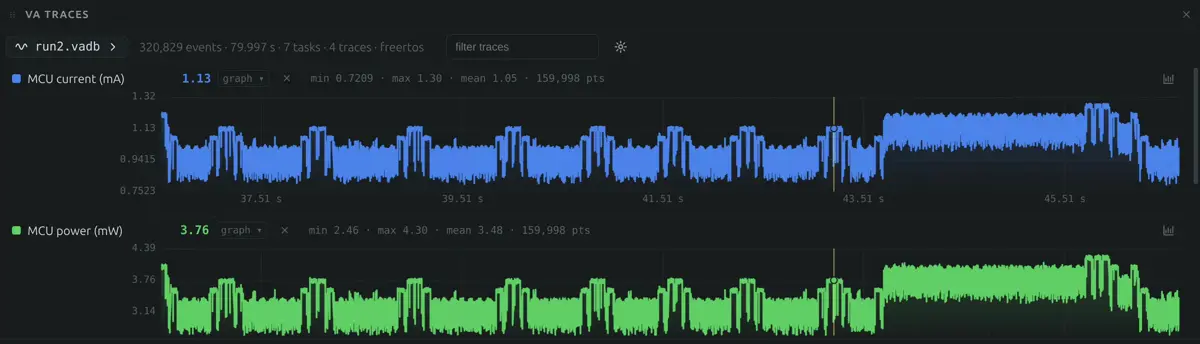
Current and power land in the capture as ordinary traces, alongside the tasks and the interrupts. Zoom, cursors, filtering and export work on them because nothing about them is a special case: 159,998 points per series, in the same file as 9.63 million instructions.
Function-level analysis
Energy in the function table
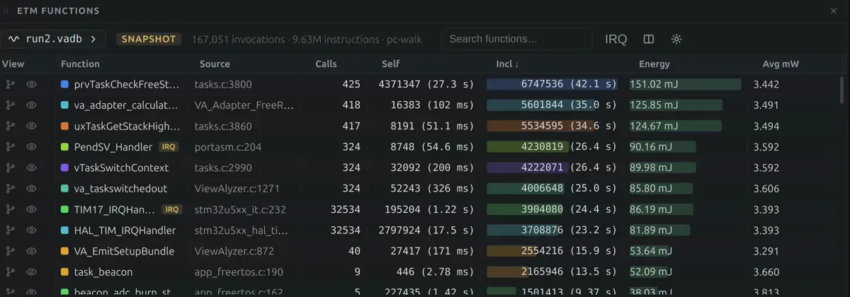
Once power shares a clock with the trace, the profiler can integrate it. Every row carries millijoules and average milliwatts next to its call count and cycles, so the slow function and the thirsty function stop being the same guess.
The first run said something we would not have guessed. The most expensive function in 45 seconds was the kernel's stack watermark walk, at 111.6 mJ, and it got there while drawing less instantaneous power than the context switch path it runs inside: 2.86 mW against 3.02 mW. Cheap every time it runs, expensive in aggregate. A time profiler prices that wrong, and so does a power meter on its own.
The arithmetic checks against the raw instrument: 127.8 mJ integrated over 45 s is 2.84 mW average, and the Joulescope's own mean for the same window is 2.79 mW.