
Engineering studies
Field notes
Two studies from our own bench: synchronizing power measurements with instruction trace, and using runtime recordings to check for regressions on real hardware.
Study 01 · Energy profiling
Power and instruction trace on a shared timeline
This entry is ours. It started with a question no hardware on the desk could answer: how many millijoules did that function cost? A Joulescope JS320 went in series with the rail of an STM32U575 running FreeRTOS. Neither instrument was built to be joined to the other, and there was no vendor to ask.
Because we own the probe, we did not have to wait for anyone. We took it in two passes: first a software sync that needs no new hardware and works with anyone's probe, then a trigger input on our own probe's FPGA that tightened the alignment by close to ten times. Idea to fused recording on hardware: one day.
- Target
- STM32U575 Nucleo · FreeRTOS · ETM trace
- Instruments
- BKPT probe (SWD + ETM) · JS320 at 1 Msps
- Method
- Trigger edges latched in hardware at 50 MHz
- Alignment
- 10.6 us rms hardware-triggered · 99.6 us rms software-synced
- Outcome
- Energy attributed per function, from one file
Nothing here is specific to Joulescope. A scope, a logic analyzer, an RF sniffer, a robot's own log stream: give it a wire and a timestamp and it joins the same record.
Synchronization methods
No new hardware
Software synchronization
The firmware raises a pin and writes a trace event inside the same critical section, at intervals dithered by an LFSR so the pattern of gaps is a fingerprint no other stretch of the capture can imitate. The Joulescope records that edge in the same 1 Msps stream as current and power, and the merge matches mark for mark, then maps one time axis onto the other. It worked on the first bench run, and it works with any probe and any instrument that can log an edge.
99.6 us rms · 300 us max
enough to attribute energy to a task
BKPT probe prototype
Hardware trigger synchronization
Getting from a task to a single function meant taking the host out of the timing path, which is the kind of change you can only make when the probe is yours. We added a trigger input to the FPGA: an incoming edge is latched at 50 MHz against the position of the byte the trace stream is carrying at that instant. The timestamp is not a clock reading that has to be reconciled with anything later. It is a place in the recording.
It also takes your firmware out of the loop. The paired trace event and the dithered pattern are gone: the edge can come from the other instrument's own trigger output, or from the probe, which pulses a hard trace t=0 the moment a capture starts. Correlating a second instrument stops being a feature you have to build into the target.
10.6 us rms · 31.7 us max · 45/45 marks
no firmware changes · what is left is 6 ppm of crystal drift
Both figures are residuals against a pure linear fit, measured on the same 45 second capture, so they compare directly. The software route stays in the product: it is the one you use before your probe has a trigger port, or when the instrument on the other end is someone else's.
Both numbers were measured on an early prototype of the probe, not the final specified design. Treat them as the floor.
Recorded data
Current and power as trace channels
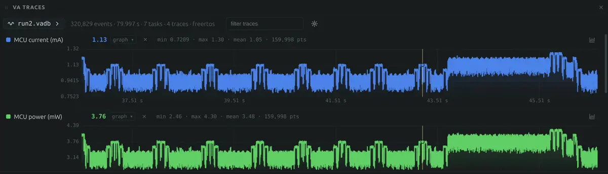
Current and power land in the capture as ordinary traces, alongside the tasks and the interrupts. Zoom, cursors, filtering and export work on them because nothing about them is a special case: 159,998 points per series, in the same file as 9.63 million instructions.
Function-level analysis
Energy in the function table
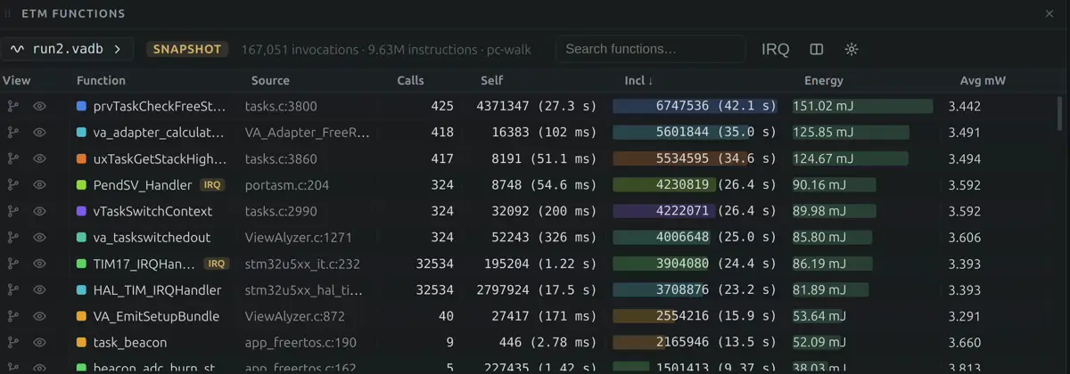
Once power shares a clock with the trace, the profiler can integrate it. Every row carries millijoules and average milliwatts next to its call count and cycles, so the slow function and the thirsty function stop being the same guess.
The first run said something we would not have guessed. The most expensive function in 45 seconds was the kernel's stack watermark walk, at 111.6 mJ, and it got there while drawing less instantaneous power than the context switch path it runs inside: 2.86 mW against 3.02 mW. Cheap every time it runs, expensive in aggregate. A time profiler prices that wrong, and so does a power meter on its own.
The arithmetic checks against the raw instrument: 127.8 mJ integrated over 45 s is 2.84 mW average, and the Joulescope's own mean for the same window is 2.79 mW.
Study 02 · Hardware regression testing
Trace-based checks in the release process
A debugger is something you reach for after the fact. An instrument runs whether or not anyone is watching. This entry is what happens when you treat the trace engine as the second thing: it is wired into our own release process, and it decides whether a change to ViewAlyzer is allowed to merge.
Every run builds firmware from the checkout under test, flashes the rack, records live trace through the headless CLI, and then asserts on the recording itself. The workload counts out loud at 100 Hz, so a single missing value is a dropped event and a failed build. The binary stamps its own identity into the trace, so stale firmware cannot produce a green run. And the scheduler numbers are compared against baselines committed to git, so a change that quietly costs a quarter of the context switches shows up as red, not as a support ticket eight months later.
These are regressions that do not exist anywhere but on silicon. No simulator has the flash wait states, the bus contention, or the interrupt that arrives one cycle early.
- Targets
- 5 Nucleo boards · ARM M3 to M33
- Matrix
- Zephyr · FreeRTOS · baremetal, across every transport and debug server each board supports
- Gate
- Zero dropped events · scheduler counts within 25% of baseline
- Evidence
- Every cell keeps its full recording, openable in the IDE
- Run
- 48 cells in 284.7 s, unattended
- Outcome
- Timing regressions caught before merge, not in the field
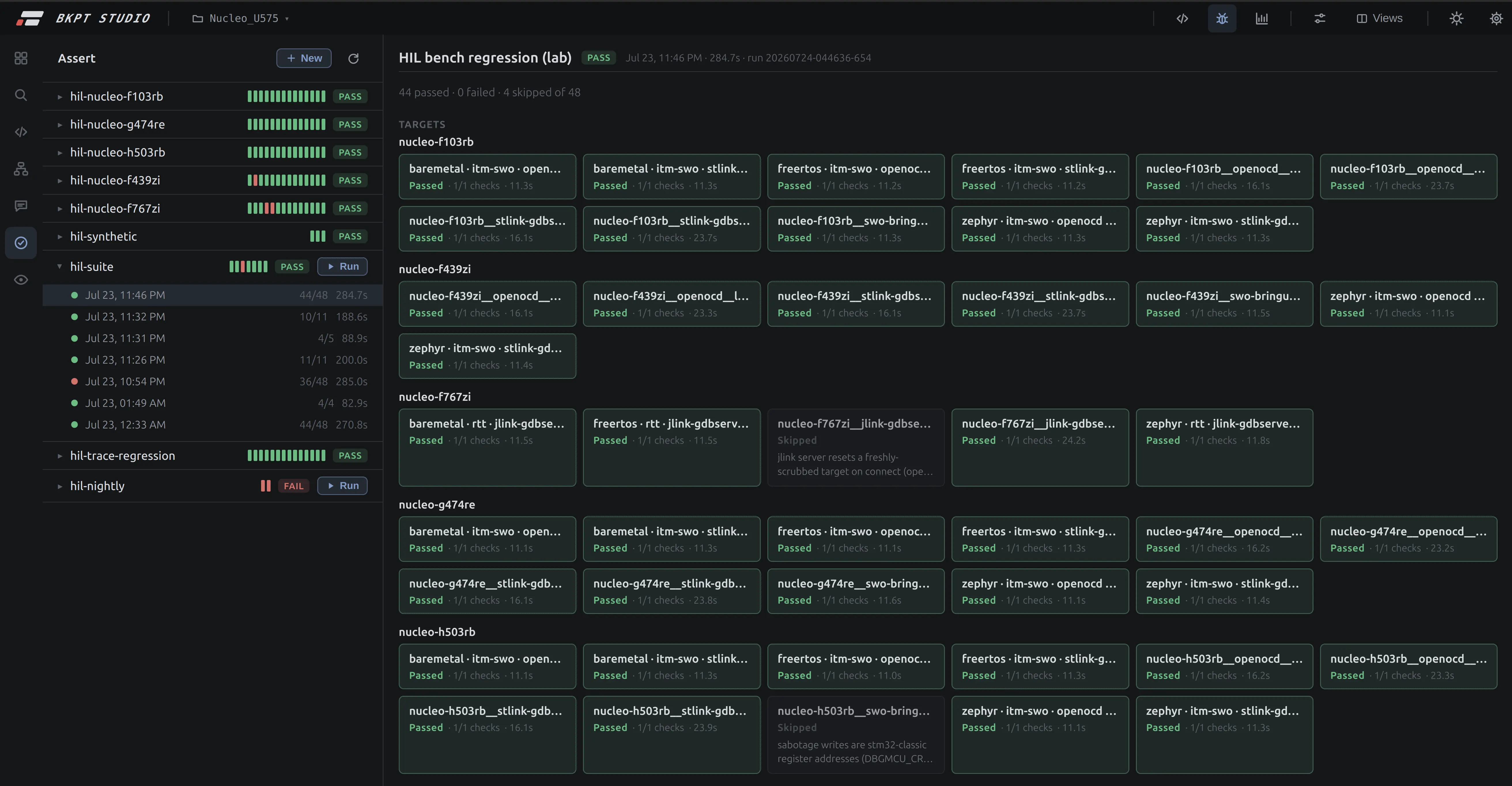
One run, as the bench reports it. Each cell is one board running one OS over one transport through one debug server. The skipped cells are not failures, they are the harness refusing to lie: it names the reason on the cell and moves on.
Evidence for each failure
A red cell is not a log line. It is a recording. Open it and you are in the same timeline you would use to debug the board by hand, at the moment the assertion broke, next to the diff that caused it.
Runtime checks in CI
Once timing is a number with a committed baseline, it is a requirement like any other. Periods, jitter, ordering, dropped events and scheduler volume all become things a pull request can break, and therefore things CI can defend.
Recordings after deployment
Turn the volume down to the events you would want at 3am and point the recorder at a ring in the device's own memory. On the bench we drain it through the probe. In the field it is your address space, so the firmware drains it itself: into flash on a fault, or up whatever radio the product already has. A returned unit stops being a guess.
SWO, RTT, a RAM ring or full ETM instruction trace. Through a J-Link, an ST-Link or our own BKPT #1 probe. The transport is a detail. What matters is that one instrument explains the system, defends it, and remembers what it did.
Evaluate on your own hardware
Try ViewAlyzer and BKPT Debug, or contact us about your application.